但如果你用同样的方法去做预测2020年的时候,发现,预测是3282亿,实际却到了 4982亿。原来2020改了规则,实际上统计的是11月1到11日的销量,理论上已经不能和历史数据合并预测,但咱们就为了图个乐,主要是为了练习一下 Python 的多项式回归和可视化绘图。
把预测先发出来:今年双十一的销量是 9029.688 亿元!坐等双十一,各位看官回来打我的脸。
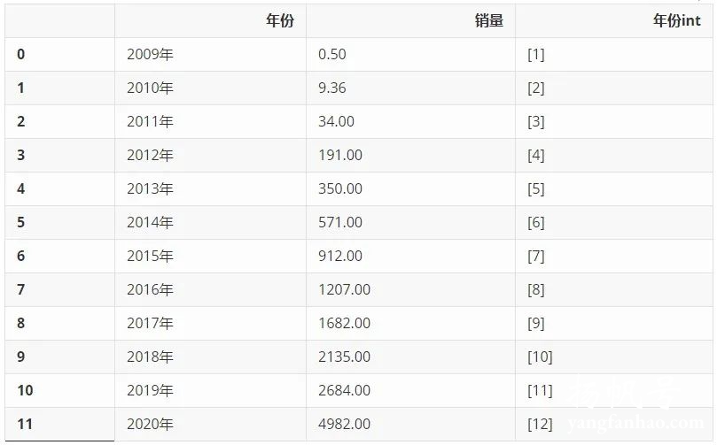
NO.01、统计历年双十一销量数据
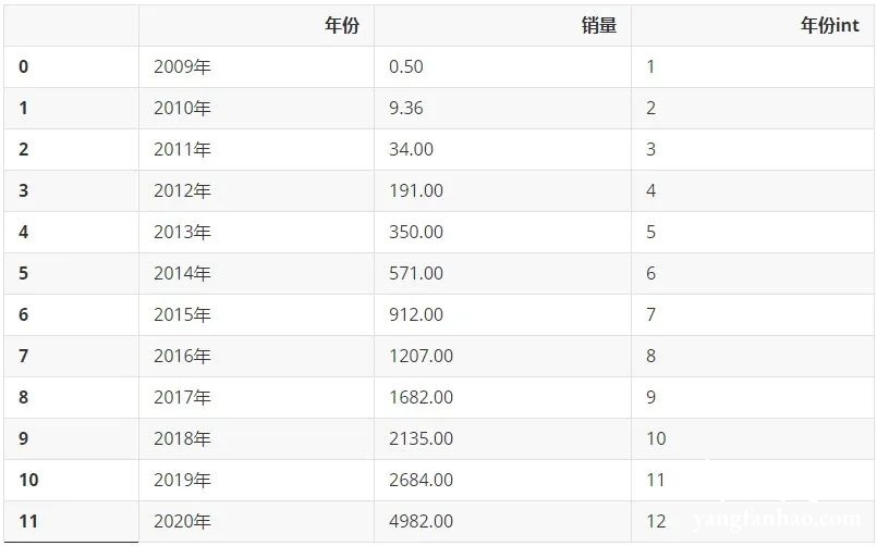
从网上搜集来历年淘宝天猫双十一销售额数据,单位为亿元,利用 Pandas 整理成 Dataframe,又添加了一列’年份int’,留作后续的计算使用。
import pandas as pd


# 数据为网络收集,历年淘宝天猫双十一销售额数据,单位为亿元,仅做示范
double11_sales = {'2009年': [0.50],
                  '2010年':[9.36],
                  '2011年':[34],
                  '2012年':[191],
                  '2013年':[350],
                  '2014年':[571],
                  '2015年':[912],
                  '2016年':[1207],
                  '2017年':[1682],
                  '2018年':[2135],
                  '2019年':[2684],
                  '2020年':[4982],
                 }


df = pd.DataFrame(double11_sales).T.reset_index()
df.rename(columns={'index':'年份',0:'销量'},inplace=True)
df['年份int'] = [[i] for i in list(range(1,len(df['年份'])+1))]
df
.dataframe tbody tr th {
vertical-align: top;
}
.dataframe thead th {
text-align: right;
}
NO.02、绘制散点图
利用 plotly 工具包,将年份对应销售量的散点图绘制出来,可以明显看到2020年的数据立马飙升。
# 散点图
import plotly as py
import plotly.graph_objs as go
import numpy as np


year = df[:]['年份']
sales = df['销量']


trace = go.Scatter(
    x=year,
    y=sales,
    mode='markers'
)
data = [trace]


layout = go.Layout(title='2009年-2020年天猫淘宝双十一历年销量')


fig = go.Figure(data=data, layout=layout)


fig.show()
<div id="2b361fe9-adc3-4cbe-810c-f76371d70c59" class="plotly-graph-div" style="height:525px; width:100%;"></div>
<script type="text/javascript">
require(["plotly"], function(Plotly) {
window.PLOTLYENV=window.PLOTLYENV || {};
if (document.getElementById("2b361fe9-adc3-4cbe-810c-f76371d70c59")) {
Plotly.newPlot(
'2b361fe9-adc3-4cbe-810c-f76371d70c59',
[{"mode": "markers", "type": "scatter", "x": ["2009u5e74", "2010u5e74", "2011u5e74", "2012u5e74", "2013u5e74", "2014u5e74", "2015u5e74", "2016u5e74", "2017u5e74", "2018u5e74", "2019u5e74", "2020u5e74"], "y": [0.5, 9.36, 34.0, 191.0, 350.0, 571.0, 912.0, 1207.0, 1682.0, 2135.0, 2684.0, 4982.0]}],
{"template": {"data": {"bar": [{"error_x": {"color": "#2a3f5f"}, "error_y": {"color": "#2a3f5f"}, "marker": {"line": {"color": "#E5ECF6", "width": 0.5}}, "type": "bar"}], "barpolar": [{"marker": {"line": {"color": "#E5ECF6", "width": 0.5}}, "type": "barpolar"}], "carpet": [{"aaxis": {"endlinecolor": "#2a3f5f", "gridcolor": "white", "linecolor": "white", "minorgridcolor": "white", "startlinecolor": "#2a3f5f"}, "baxis": {"endlinecolor": "#2a3f5f", "gridcolor": "white", "linecolor": "white", "minorgridcolor": "white", "startlinecolor": "#2a3f5f"}, "type": "carpet"}], "choropleth": [{"colorbar": {"outlinewidth": 0, "ticks": ""}, "type": "choropleth"}], "contour": [{"colorbar": {"outlinewidth": 0, "ticks": ""}, "colorscale": [[0.0, "#0d0887"], [0.1111111111111111, "#46039f"], [0.2222222222222222, "#7201a8"], [0.3333333333333333, "#9c179e"], [0.4444444444444444, "#bd3786"], [0.5555555555555556, "#d8576b"], [0.6666666666666666, "#ed7953"], [0.7777777777777778, "#fb9f3a"], [0.8888888888888888, "#fdca26"], [1.0, "#f0f921"]], "type": "contour"}], "contourcarpet": [{"colorbar": {"outlinewidth": 0, "ticks": ""}, "type": "contourcarpet"}], "heatmap": [{"colorbar": {"outlinewidth": 0, "ticks": ""}, "colorscale": [[0.0, "#0d0887"], [0.1111111111111111, "#46039f"], [0.2222222222222222, "#7201a8"], [0.3333333333333333, "#9c179e"], [0.4444444444444444, "#bd3786"], [0.5555555555555556, "#d8576b"], [0.6666666666666666, "#ed7953"], [0.7777777777777778, "#fb9f3a"], [0.8888888888888888, "#fdca26"], [1.0, "#f0f921"]], "type": "heatmap"}], "heatmapgl": [{"colorbar": {"outlinewidth": 0, "ticks": ""}, "colorscale": [[0.0, "#0d0887"], [0.1111111111111111, "#46039f"], [0.2222222222222222, "#7201a8"], [0.3333333333333333, "#9c179e"], [0.4444444444444444, "#bd3786"], [0.5555555555555556, "#d8576b"], [0.6666666666666666, "#ed7953"], [0.7777777777777778, "#fb9f3a"], [0.8888888888888888, "#fdca26"], [1.0, "#f0f921"]], "type": "heatmapgl"}], "histogram": [{"marker": {"colorbar": {"outlinewidth": 0, "ticks": ""}}, "type": "histogram"}], "histogram2d": [{"colorbar": {"outlinewidth": 0, "ticks": ""}, "colorscale": [[0.0, "#0d0887"], [0.1111111111111111, "#46039f"], [0.2222222222222222, "#7201a8"], [0.3333333333333333, "#9c179e"], [0.4444444444444444, "#bd3786"], [0.5555555555555556, "#d8576b"], [0.6666666666666666, "#ed7953"], [0.7777777777777778, "#fb9f3a"], [0.8888888888888888, "#fdca26"], [1.0, "#f0f921"]], "type": "histogram2d"}], "histogram2dcontour": [{"colorbar": {"outlinewidth": 0, "ticks": ""}, "colorscale": [[0.0, "#0d0887"], [0.1111111111111111, "#46039f"], [0.2222222222222222, "#7201a8"], [0.3333333333333333, "#9c179e"], [0.4444444444444444, "#bd3786"], [0.5555555555555556, "#d8576b"], [0.6666666666666666, "#ed7953"], [0.7777777777777778, "#fb9f3a"], [0.8888888888888888, "#fdca26"], [1.0, "#f0f921"]], "type": "histogram2dcontour"}], "mesh3d": [{"colorbar": {"outlinewidth": 0, "ticks": ""}, "type": "mesh3d"}], "parcoords": [{"line": {"colorbar": {"outlinewidth": 0, "ticks": ""}}, "type": "parcoords"}], "pie": [{"automargin": true, "type": "pie"}], "scatter": [{"marker": {"colorbar": {"outlinewidth": 0, "ticks": ""}}, "type": "scatter"}], "scatter3d": [{"line": {"colorbar": {"outlinewidth": 0, "ticks": ""}}, "marker": {"colorbar": {"outlinewidth": 0, "ticks": ""}}, "type": "scatter3d"}], "scattercarpet": [{"marker": {"colorbar": {"outlinewidth": 0, "ticks": ""}}, "type": "scattercarpet"}], "scattergeo": [{"marker": {"colorbar": {"outlinewidth": 0, "ticks": ""}}, "type": "scattergeo"}], "scattergl": [{"marker": {"colorbar": {"outlinewidth": 0, "ticks": ""}}, "type": "scattergl"}], "scattermapbox": [{"marker": {"colorbar": {"outlinewidth": 0, "ticks": ""}}, "type": "scattermapbox"}], "scatterpolar": [{"marker": {"colorbar": {"outlinewidth": 0, "ticks": ""}}, "type": "scatterpolar"}], "scatterpolargl": [{"marker": {"colorbar": {"outlinewidth": 0, "ticks": ""}}, "type": "scatterpolargl"}], "scatterternary": [{"marker": {"colorbar": {"outlinewidth": 0, "ticks": ""}}, "type": "scatterternary"}], "surface": [{"colorbar": {"outlinewidth": 0, "ticks": ""}, "colorscale": [[0.0, "#0d0887"], [0.1111111111111111, "#46039f"], [0.2222222222222222, "#7201a8"], [0.3333333333333333, "#9c179e"], [0.4444444444444444, "#bd3786"], [0.5555555555555556, "#d8576b"], [0.6666666666666666, "#ed7953"], [0.7777777777777778, "#fb9f3a"], [0.8888888888888888, "#fdca26"], [1.0, "#f0f921"]], "type": "surface"}], "table": [{"cells": {"fill": {"color": "#EBF0F8"}, "line": {"color": "white"}}, "header": {"fill": {"color": "#C8D4E3"}, "line": {"color": "white"}}, "type": "table"}]}, "layout": {"annotationdefaults": {"arrowcolor": "#2a3f5f", "arrowhead": 0, "arrowwidth": 1}, "coloraxis": {"colorbar": {"outlinewidth": 0, "ticks": ""}}, "colorscale": {"diverging": [[0, "#8e0152"], [0.1, "#c51b7d"], [0.2, "#de77ae"], [0.3, "#f1b6da"], [0.4, "#fde0ef"], [0.5, "#f7f7f7"], [0.6, "#e6f5d0"], [0.7, "#b8e186"], [0.8, "#7fbc41"], [0.9, "#4d9221"], [1, "#276419"]], "sequential": [[0.0, "#0d0887"], [0.1111111111111111, "#46039f"], [0.2222222222222222, "#7201a8"], [0.3333333333333333, "#9c179e"], [0.4444444444444444, "#bd3786"], [0.5555555555555556, "#d8576b"], [0.6666666666666666, "#ed7953"], [0.7777777777777778, "#fb9f3a"], [0.8888888888888888, "#fdca26"], [1.0, "#f0f921"]], "sequentialminus": [[0.0, "#0d0887"], [0.1111111111111111, "#46039f"], [0.2222222222222222, "#7201a8"], [0.3333333333333333, "#9c179e"], [0.4444444444444444, "#bd3786"], [0.5555555555555556, "#d8576b"], [0.6666666666666666, "#ed7953"], [0.7777777777777778, "#fb9f3a"], [0.8888888888888888, "#fdca26"], [1.0, "#f0f921"]]}, "colorway": ["#636efa", "#EF553B", "#00cc96", "#ab63fa", "#FFA15A", "#19d3f3", "#FF6692", "#B6E880", "#FF97FF", "#FECB52"], "font": {"color": "#2a3f5f"}, "geo": {"bgcolor": "white", "lakecolor": "white", "landcolor": "#E5ECF6", "showlakes": true, "showland": true, "subunitcolor": "white"}, "hoverlabel": {"align": "left"}, "hovermode": "closest", "mapbox": {"style": "light"}, "paper_bgcolor": "white", "plot_bgcolor": "#E5ECF6", "polar": {"angularaxis": {"gridcolor": "white", "linecolor": "white", "ticks": ""}, "bgcolor": "#E5ECF6", "radialaxis": {"gridcolor": "white", "linecolor": "white", "ticks": ""}}, "scene": {"xaxis": {"backgroundcolor": "#E5ECF6", "gridcolor": "white", "gridwidth": 2, "linecolor": "white", "showbackground": true, "ticks": "", "zerolinecolor": "white"}, "yaxis": {"backgroundcolor": "#E5ECF6", "gridcolor": "white", "gridwidth": 2, "linecolor": "white", "showbackground": true, "ticks": "", "zerolinecolor": "white"}, "zaxis": {"backgroundcolor": "#E5ECF6", "gridcolor": "white", "gridwidth": 2, "linecolor": "white", "showbackground": true, "ticks": "", "zerolinecolor": "white"}}, "shapedefaults": {"line": {"color": "#2a3f5f"}}, "ternary": {"aaxis": {"gridcolor": "white", "linecolor": "white", "ticks": ""}, "baxis": {"gridcolor": "white", "linecolor": "white", "ticks": ""}, "bgcolor": "#E5ECF6", "caxis": {"gridcolor": "white", "linecolor": "white", "ticks": ""}}, "title": {"x": 0.05}, "xaxis": {"automargin": true, "gridcolor": "white", "linecolor": "white", "ticks": "", "title": {"standoff": 15}, "zerolinecolor": "white", "zerolinewidth": 2}, "yaxis": {"automargin": true, "gridcolor": "white", "linecolor": "white", "ticks": "", "title": {"standoff": 15}, "zerolinecolor": "white", "zerolinewidth": 2}}}, "title": {"text": "2009u5e74-2020u5e74u5929u732bu6dd8u5b9du53ccu5341u4e00u5386u5e74u9500u91cf"}},
{"responsive": true}
).then(function(){var gd = document.getElementById('2b361fe9-adc3-4cbe-810c-f76371d70c59');
var x = new MutationObserver(function (mutations, observer) {{
var display = window.getComputedStyle(gd).display;
if (!display || display === 'none') {{
console.log([gd, 'removed!']);
Plotly.purge(gd);
observer.disconnect();
}}
}});
// Listen for the removal of the full notebook cells
var notebookContainer = gd.closest('#notebook-container');
if (notebookContainer) {{
x.observe(notebookContainer, {childList: true});
}}
// Listen for the clearing of the current output cell
var outputEl = gd.closest('.output');
if (outputEl) {{
x.observe(outputEl, {childList: true});
}} })
};
});
</script>
</div>
NO.03、引入 Scikit-Learn 库搭建模型
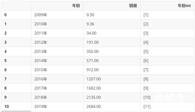
一元多次线性回归
我们先来回顾一下2009-2019年的数据多么美妙。先只选取2009-2019年的数据:
df_2009_2019 = df[:-1]
df_2009_2019
.dataframe tbody tr th {
vertical-align: top;
}
.dataframe thead th {
text-align: right;
}
通过以下代码生成二次项数据:
from sklearn.preprocessing import PolynomialFeatures
poly_reg = PolynomialFeatures(degree=2)
X_ = poly_reg.fit_transform(list(df_2009_2019['年份int']))
1.第一行代码引入用于增加一个多次项内容的模块 PolynomialFeatures
2.第二行代码设置最高次项为二次项,为生成二次项数据(x平方)做准备
3.第三行代码将原有的X转换为一个新的二维数组X_,该二维数据包含新生成的二次项数据(x平方)和原有的一次项数据(x)
X_ 的内容为下方代码所示的一个二维数组,其中第一列数据为常数项(其实就是X的0次方),没有特殊含义,对分析结果不会产生影响;第二列数据为原有的一次项数据(x);第三列数据为新生成的二次项数据(x的平方)。
X_array([[ 1., 1., 1.],
[ 1., 2., 4.],
[ 1., 3., 9.],
[ 1., 4., 16.],
[ 1., 5., 25.],
[ 1., 6., 36.],
[ 1., 7., 49.],
[ 1., 8., 64.],
[ 1., 9., 81.],
[ 1., 10., 100.],
[ 1., 11., 121.]])from sklearn.linear_model import LinearRegression
regr = LinearRegression()
regr.fit(X_,list(df_2009_2019['销量']))LinearRegression()1.第一行代码从 Scikit-Learn 库引入线性回归的相关模块 LinearRegression;
2.第二行代码构造一个初始的线性回归模型并命名为 regr;
3.第三行代码用fit() 函数完成模型搭建,此时的regr就是一个搭建好的线性回归模型。
NO.04、模型预测
接下来就可以利用搭建好的模型 regr 来预测数据。加上自变量是12,那么使用 predict() 函数就能预测对应的因变量有,代码如下:
XX_ = poly_reg.fit_transform([[12]])XX_array([[ 1., 12., 144.]])y = regr.predict(XX_)
yarray([3282.23478788])这里我们就得到了如果按照这个趋势2009-2019的趋势预测2020的结果,就是3282,但实际却是4982亿,原因就是上文提到的合并计算了,金额一下子变大了,绘制成图,就是下面这样:
# 散点图
import plotly as py
import plotly.graph_objs as go
import numpy as np
year = list(df['年份'])
sales = df['销量']
trace1 = go.Scatter(
x=year,
y=sales,
mode='markers',
name="实际销量"       # 第一个图例名称
)
XX_ = poly_reg.fit_transform(list(df['年份int'])+[[13]])
regr = LinearRegression()
regr.fit(X_,list(df_2009_2019['销量']))
trace2 = go.Scatter(
x=list(df['年份']),
y=regr.predict(XX_),
mode='lines',
name="拟合数据",  # 第2个图例名称
)
data = [trace1,trace2]
layout = go.Layout(title='天猫淘宝双十一历年销量',
xaxis_title='年份',
yaxis_title='销量')
fig = go.Figure(data=data, layout=layout)
fig.show()-var gd = document.getElementById('e8ae9262-7d14-4b38-b661-fb79f13ff6a7');
var x = new MutationObserver(function (mutations, observer) {{
var display = window.getComputedStyle(gd).display;
if (!display || display === 'none') {{
console.log([gd, 'removed!']);
Plotly.purge(gd);
observer.disconnect();
}}
}});
// Listen for the removal of the full notebook cells
var notebookContainer = gd.closest('#notebook-container');
if (notebookContainer) {{
x.observe(notebookContainer, {childList: true});
}}
// Listen for the clearing of the current output cell
var outputEl = gd.closest('.output');
if (outputEl) {{
x.observe(outputEl, {childList: true});
}} })
};
});
</script>
</div>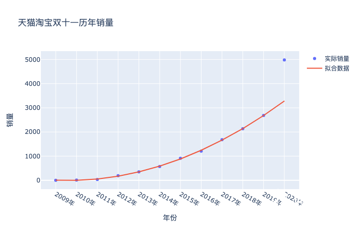
NO.05、预测2021年的销量
既然数据发生了巨大的偏离,咱们也别深究了,就大力出奇迹。同样的方法,把2020年的真实数据纳入进来,二话不说拟合一样,看看会得到什么结果:
from sklearn.preprocessing import PolynomialFeatures
poly_reg = PolynomialFeatures(degree=5)
X_ = poly_reg.fit_transform(list(df['年份int']))
## 预测2020年
regr = LinearRegression()
regr.fit(X_,list(df['销量']))LinearRegression()XXX_ = poly_reg.fit_transform(list(df['年份int'])+[[13]])# 散点图
import plotly as py
import plotly.graph_objs as go
import numpy as np
year = list(df['年份'])
sales = df['销量']
trace1 = go.Scatter(
x=year+['2021年','2022年','2023年'],
y=sales,
mode='markers',
name="实际销量" # 第一个图例名称
)
trace2 = go.Scatter(
x=year+['2021年','2022年','2023年'],
y=regr.predict(XXX_),
mode='lines',
name="预测销量" # 第一个图例名称
)
trace3 = go.Scatter(
x=['2021年'],
y=[regr.predict(XXX_)[-1]],
mode='markers',
name="2021年预测销量" # 第一个图例名称
)
data = [trace1,trace2,trace3]
layout = go.Layout(title='天猫淘宝双十一历年销量',
xaxis_title='年份',
yaxis_title='销量')
fig = go.Figure(data=data, layout=layout)
fig.show() <div id="3151a044-f334-4544-8e20-b4908350e140" class="plotly-graph-div" style="height:525px; width:100%;"></div>
<script type="text/javascript">
require(["plotly"], function(Plotly) {
window.PLOTLYENV=window.PLOTLYENV || {};
if (document.getElementById("3151a044-f334-4544-8e20-b4908350e140")) {
Plotly.newPlot(
'3151a044-f334-4544-8e20-b4908350e140',
[{"mode": "markers", "name": "u5b9eu9645u9500u91cf", "type": "scatter", "x": ["2009u5e74", "2010u5e74", "2011u5e74", "2012u5e74", "2013u5e74", "2014u5e74", "2015u5e74", "2016u5e74", "2017u5e74", "2018u5e74", "2019u5e74", "2020u5e74", "2021u5e74", "2022u5e74", "2023u5e74"], "y": [0.5, 9.36, 34.0, 191.0, 350.0, 571.0, 912.0, 1207.0, 1682.0, 2135.0, 2684.0, 4982.0]}, {"mode": "lines", "name": "u9884u6d4bu9500u91cf", "type": "scatter", "x": ["2009u5e74", "2010u5e74", "2011u5e74", "2012u5e74", "2013u5e74", "2014u5e74", "2015u5e74", "2016u5e74", "2017u5e74", "2018u5e74", "2019u5e74", "2020u5e74", "2021u5e74", "2022u5e74", "2023u5e74"], "y": [-31.73938915412782, 84.24415467459653, 47.98135953421206, 98.6884039599804, 304.45773756556355, 625.1325380574217, 975.1811682492444, 1286.5716330763207, 1571.64603660996, 1985.995039071935, 2891.332313848736, 4918.369004506214, 9029.688181803827]}, {"mode": "markers", "name": "2021u5e74u9884u6d4bu9500u91cf", "type": "scatter", "x": ["2021u5e74"], "y": [9029.688181803827]}],
{"template": {"data": {"bar": [{"error_x": {"color": "#2a3f5f"}, "error_y": {"color": "#2a3f5f"}, "marker": {"line": {"color": "#E5ECF6", "width": 0.5}}, "type": "bar"}], "barpolar": [{"marker": {"line": {"color": "#E5ECF6", "width": 0.5}}, "type": "barpolar"}], "carpet": [{"aaxis": {"endlinecolor": "#2a3f5f", "gridcolor": "white", "linecolor": "white", "minorgridcolor": "white", "startlinecolor": "#2a3f5f"}, "baxis": {"endlinecolor": "#2a3f5f", "gridcolor": "white", "linecolor": "white", "minorgridcolor": "white", "startlinecolor": "#2a3f5f"}, "type": "carpet"}], "choropleth": [{"colorbar": {"outlinewidth": 0, "ticks": ""}, "type": "choropleth"}], "contour": [{"colorbar": {"outlinewidth": 0, "ticks": ""}, "colorscale": [[0.0, "#0d0887"], [0.1111111111111111, "#46039f"], [0.2222222222222222, "#7201a8"], [0.3333333333333333, "#9c179e"], [0.4444444444444444, "#bd3786"], [0.5555555555555556, "#d8576b"], [0.6666666666666666, "#ed7953"], [0.7777777777777778, "#fb9f3a"], [0.8888888888888888, "#fdca26"], [1.0, "#f0f921"]], "type": "contour"}], "contourcarpet": [{"colorbar": {"outlinewidth": 0, "ticks": ""}, "type": "contourcarpet"}], "heatmap": [{"colorbar": {"outlinewidth": 0, "ticks": ""}, "colorscale": [[0.0, "#0d0887"], [0.1111111111111111, "#46039f"], [0.2222222222222222, "#7201a8"], [0.3333333333333333, "#9c179e"], [0.4444444444444444, "#bd3786"], [0.5555555555555556, "#d8576b"], [0.6666666666666666, "#ed7953"], [0.7777777777777778, "#fb9f3a"], [0.8888888888888888, "#fdca26"], [1.0, "#f0f921"]], "type": "heatmap"}], "heatmapgl": [{"colorbar": {"outlinewidth": 0, "ticks": ""}, "colorscale": [[0.0, "#0d0887"], [0.1111111111111111, "#46039f"], [0.2222222222222222, "#7201a8"], [0.3333333333333333, "#9c179e"], [0.4444444444444444, "#bd3786"], [0.5555555555555556, "#d8576b"], [0.6666666666666666, "#ed7953"], [0.7777777777777778, "#fb9f3a"], [0.8888888888888888, "#fdca26"], [1.0, "#f0f921"]], "type": "heatmapgl"}], "histogram": [{"marker": {"colorbar": {"outlinewidth": 0, "ticks": ""}}, "type": "histogram"}], "histogram2d": [{"colorbar": {"outlinewidth": 0, "ticks": ""}, "colorscale": [[0.0, "#0d0887"], [0.1111111111111111, "#46039f"], [0.2222222222222222, "#7201a8"], [0.3333333333333333, "#9c179e"], [0.4444444444444444, "#bd3786"], [0.5555555555555556, "#d8576b"], [0.6666666666666666, "#ed7953"], [0.7777777777777778, "#fb9f3a"], [0.8888888888888888, "#fdca26"], [1.0, "#f0f921"]], "type": "histogram2d"}], "histogram2dcontour": [{"colorbar": {"outlinewidth": 0, "ticks": ""}, "colorscale": [[0.0, "#0d0887"], [0.1111111111111111, "#46039f"], [0.2222222222222222, "#7201a8"], [0.3333333333333333, "#9c179e"], [0.4444444444444444, "#bd3786"], [0.5555555555555556, "#d8576b"], [0.6666666666666666, "#ed7953"], [0.7777777777777778, "#fb9f3a"], [0.8888888888888888, "#fdca26"], [1.0, "#f0f921"]], "type": "histogram2dcontour"}], "mesh3d": [{"colorbar": {"outlinewidth": 0, "ticks": ""}, "type": "mesh3d"}], "parcoords": [{"line": {"colorbar": {"outlinewidth": 0, "ticks": ""}}, "type": "parcoords"}], "pie": [{"automargin": true, "type": "pie"}], "scatter": [{"marker": {"colorbar": {"outlinewidth": 0, "ticks": ""}}, "type": "scatter"}], "scatter3d": [{"line": {"colorbar": {"outlinewidth": 0, "ticks": ""}}, "marker": {"colorbar": {"outlinewidth": 0, "ticks": ""}}, "type": "scatter3d"}], "scattercarpet": [{"marker": {"colorbar": {"outlinewidth": 0, "ticks": ""}}, "type": "scattercarpet"}], "scattergeo": [{"marker": {"colorbar": {"outlinewidth": 0, "ticks": ""}}, "type": "scattergeo"}], "scattergl": [{"marker": {"colorbar": {"outlinewidth": 0, "ticks": ""}}, "type": "scattergl"}], "scattermapbox": [{"marker": {"colorbar": {"outlinewidth": 0, "ticks": ""}}, "type": "scattermapbox"}], "scatterpolar": [{"marker": {"colorbar": {"outlinewidth": 0, "ticks": ""}}, "type": "scatterpolar"}], "scatterpolargl": [{"marker": {"colorbar": {"outlinewidth": 0, "ticks": ""}}, "type": "scatterpolargl"}], "scatterternary": [{"marker": {"colorbar": {"outlinewidth": 0, "ticks": ""}}, "type": "scatterternary"}], "surface": [{"colorbar": {"outlinewidth": 0, "ticks": ""}, "colorscale": [[0.0, "#0d0887"], [0.1111111111111111, "#46039f"], [0.2222222222222222, "#7201a8"], [0.3333333333333333, "#9c179e"], [0.4444444444444444, "#bd3786"], [0.5555555555555556, "#d8576b"], [0.6666666666666666, "#ed7953"], [0.7777777777777778, "#fb9f3a"], [0.8888888888888888, "#fdca26"], [1.0, "#f0f921"]], "type": "surface"}], "table": [{"cells": {"fill": {"color": "#EBF0F8"}, "line": {"color": "white"}}, "header": {"fill": {"color": "#C8D4E3"}, "line": {"color": "white"}}, "type": "table"}]}, "layout": {"annotationdefaults": {"arrowcolor": "#2a3f5f", "arrowhead": 0, "arrowwidth": 1}, "coloraxis": {"colorbar": {"outlinewidth": 0, "ticks": ""}}, "colorscale": {"diverging": [[0, "#8e0152"], [0.1, "#c51b7d"], [0.2, "#de77ae"], [0.3, "#f1b6da"], [0.4, "#fde0ef"], [0.5, "#f7f7f7"], [0.6, "#e6f5d0"], [0.7, "#b8e186"], [0.8, "#7fbc41"], [0.9, "#4d9221"], [1, "#276419"]], "sequential": [[0.0, "#0d0887"], [0.1111111111111111, "#46039f"], [0.2222222222222222, "#7201a8"], [0.3333333333333333, "#9c179e"], [0.4444444444444444, "#bd3786"], [0.5555555555555556, "#d8576b"], [0.6666666666666666, "#ed7953"], [0.7777777777777778, "#fb9f3a"], [0.8888888888888888, "#fdca26"], [1.0, "#f0f921"]], "sequentialminus": [[0.0, "#0d0887"], [0.1111111111111111, "#46039f"], [0.2222222222222222, "#7201a8"], [0.3333333333333333, "#9c179e"], [0.4444444444444444, "#bd3786"], [0.5555555555555556, "#d8576b"], [0.6666666666666666, "#ed7953"], [0.7777777777777778, "#fb9f3a"], [0.8888888888888888, "#fdca26"], [1.0, "#f0f921"]]}, "colorway": ["#636efa", "#EF553B", "#00cc96", "#ab63fa", "#FFA15A", "#19d3f3", "#FF6692", "#B6E880", "#FF97FF", "#FECB52"], "font": {"color": "#2a3f5f"}, "geo": {"bgcolor": "white", "lakecolor": "white", "landcolor": "#E5ECF6", "showlakes": true, "showland": true, "subunitcolor": "white"}, "hoverlabel": {"align": "left"}, "hovermode": "closest", "mapbox": {"style": "light"}, "paper_bgcolor": "white", "plot_bgcolor": "#E5ECF6", "polar": {"angularaxis": {"gridcolor": "white", "linecolor": "white", "ticks": ""}, "bgcolor": "#E5ECF6", "radialaxis": {"gridcolor": "white", "linecolor": "white", "ticks": ""}}, "scene": {"xaxis": {"backgroundcolor": "#E5ECF6", "gridcolor": "white", "gridwidth": 2, "linecolor": "white", "showbackground": true, "ticks": "", "zerolinecolor": "white"}, "yaxis": {"backgroundcolor": "#E5ECF6", "gridcolor": "white", "gridwidth": 2, "linecolor": "white", "showbackground": true, "ticks": "", "zerolinecolor": "white"}, "zaxis": {"backgroundcolor": "#E5ECF6", "gridcolor": "white", "gridwidth": 2, "linecolor": "white", "showbackground": true, "ticks": "", "zerolinecolor": "white"}}, "shapedefaults": {"line": {"color": "#2a3f5f"}}, "ternary": {"aaxis": {"gridcolor": "white", "linecolor": "white", "ticks": ""}, "baxis": {"gridcolor": "white", "linecolor": "white", "ticks": ""}, "bgcolor": "#E5ECF6", "caxis": {"gridcolor": "white", "linecolor": "white", "ticks": ""}}, "title": {"x": 0.05}, "xaxis": {"automargin": true, "gridcolor": "white", "linecolor": "white", "ticks": "", "title": {"standoff": 15}, "zerolinecolor": "white", "zerolinewidth": 2}, "yaxis": {"automargin": true, "gridcolor": "white", "linecolor": "white", "ticks": "", "title": {"standoff": 15}, "zerolinecolor": "white", "zerolinewidth": 2}}}, "title": {"text": "u5929u732bu6dd8u5b9du53ccu5341u4e00u5386u5e74u9500u91cf"}, "xaxis": {"title": {"text": "u5e74u4efd"}}, "yaxis": {"title": {"text": "u9500u91cf"}}},
{"responsive": true}
).then(function(){var gd = document.getElementById('3151a044-f334-4544-8e20-b4908350e140');
var x = new MutationObserver(function (mutations, observer) {{
var display = window.getComputedStyle(gd).display;
if (!display || display === 'none') {{
console.log([gd, 'removed!']);
Plotly.purge(gd);
observer.disconnect();
}}
}});
// Listen for the removal of the full notebook cells
var notebookContainer = gd.closest('#notebook-container');
if (notebookContainer) {{
x.observe(notebookContainer, {childList: true});
}}
// Listen for the clearing of the current output cell
var outputEl = gd.closest('.output');
if (outputEl) {{
x.observe(outputEl, {childList: true});
}} })
};
});
</script>
</div>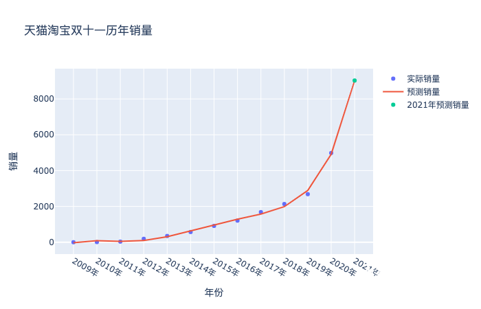
NO.06、多项式预测的次数到底如何选择
在选择模型中的次数方面,可以通过设置程序,循环计算各个次数下预测误差,然后再根据结果反选参数。
df_new = df.copy()
df_new['年份int'] = df['年份int'].apply(lambda x: x[0])
df_new
.dataframe tbody tr th {
vertical-align: top;
}
.dataframe thead th {
text-align: right;
}
#  多项式回归预测次数选择
# 计算 m 次多项式回归预测结果的 MSE 评价指标并绘图
from sklearn.pipeline import make_pipeline
from sklearn.metrics import mean_squared_error
train_df = df_new[:int(len(df)*0.95)]
test_df = df_new[int(len(df)*0.5):]
# 定义训练和测试使用的自变量和因变量
train_x = train_df['年份int'].values
train_y = train_df['销量'].values
# print(train_x)
test_x = test_df['年份int'].values
test_y = test_df['销量'].values
train_x = train_x.reshape(len(train_x),1)
test_x = test_x.reshape(len(test_x),1)
train_y = train_y.reshape(len(train_y),1)
mse = [] # 用于存储各最高次多项式 MSE 值
m = 1 # 初始 m 值
m_max = 10 # 设定最高次数
while m <= m_max:
model = make_pipeline(PolynomialFeatures(m, include_bias=False), LinearRegression())
model.fit(train_x, train_y) # 训练模型
pre_y = model.predict(test_x) # 测试模型
mse.append(mean_squared_error(test_y, pre_y.flatten())) # 计算 MSE
m = m + 1
print("MSE 计算结果: ", mse)
# 绘图
plt.plot([i for i in range(1, m_max + 1)], mse, 'r')
plt.scatter([i for i in range(1, m_max + 1)], mse)
# 绘制图名称等
plt.title("MSE of m degree of polynomial regression")
plt.xlabel("m")
plt.ylabel("MSE")
MSE 计算结果: [1088092.9621201046, 481951.27857828484, 478840.8575107471, 477235.9140442428, 484657.87153138855, 509758.1526412842, 344204.1969956556, 429874.9229308078, 8281846.231771571, 146298201.8473966]Text(0, 0.5, 'MSE')
从误差结果可以看到,次数取2到8误差基本稳定,没有明显的减少了,但其实你试试就知道,次数选择3的时候,预测的销量是6213亿元,次数选择5的时候,预测的销量是9029亿元,对于销售量来说,这个范围已经够大的了。我也就斗胆猜到9029亿元,我的胆量也就预测到这里了,破万亿就太夸张了,欢迎胆子大的同学留下你们的预测结果,让我们11月11日,拭目以待吧。
NO.07、总结最后
希望这篇文章带着对 Python 的多项式回归和 Plotly可视化绘图还不熟悉的同学一起练习一下。
本文出品:CDA数据分析师